anlak.com

Rectangle Blanket Problem

, Friday 2 August 2019
Here is our paper titled "Rectangle Blanket Problem: Binary integer linear programming formulation and solution algorithms", so google scholar can finally index the pdf.

In layman's terms, we are given a shape and we are trying to put K non-overlapping rectangles that best represents the shape.

Click here to download the paper.

Warm start linear programs with Gurobi

, Saturday 17 September 2016
The Gurobi documentation is a little bit confusing about warm starting linear programs. Warm start is sometimes referred as advanced start. I decided to gather everything about it in a single post because recently a colleague had the same issue. Especially if you are applying column generation you should warm start your linear programs at each iteration to significantly speed up the optimization.

The Problem

Assume you have a linear programming model and called optimize() on the model. Now you want to slightly modify your model and use the previous solution as an initial starting point to speed things up. This is called warm start.

Gurobi would do a warm start in certain cases, you don't need to do any extra work. When you change
  • variable bounds
  • coefficients in the objective value
  • right hand side of the constraints
  • coefficients of variables in the constraints
Gurobi will do a warm start automatically.

However, when you
  • add/remove a variable
  • add/remove a constraint
Gurobi will discard the previous solution and start optimizing from scratch.

The remedy

There are two different ways of achieving warm start:
  • Setting primal and dual variables values using PStart and DStart attributes.
  • Setting the simplex basic using VBasis and CBasis attributes. (CBasis corresponds to slack variables if you were wondering)
Whichever method you choose, you need to store the corresponding values before modifying the model. Then restore these values after the modification.

According to Gurobi documentation using VBasis/CBasis method performs better. This is almost always true. However, in my comparisons PStart/DStart method led to increased speed gains for my model. Although I can't exactly explain why this happens, I suspect it has something to do with my problem structure. See the discussion here if you are interested. To summarize, you should check which warm start method works best for you. If you are lazy, use the VBasis/CBasis method.

Below I give code snippets on how to store and load relevant values for each method. There is also GitHub repo available for the full code. The code is written in Java but you will get the idea.

PStart/DStart

First save the actual values for both primal and dual variables:
PSTARTS = new double[vars.length];
for (int i = 0; i < vars.length; i++)
  PSTARTS[i] = vars[i].get(DoubleAttr.X);

DSTARTS = new double[constrs.length];
for (int i = 0; i < constrs.length; i++)
  DSTARTS[i] = constrs[i].get(DoubleAttr.Pi);
After modifying the model load variable values using PStart/DStart attributes:
for (int i = 0; i < vars.length; i++)
  vars[i].set(PStart, PSTARTS[i]);
for (int i = 0; i < constrs.length; i++)
  constrs[i].set(DStart, DSTARTS[i]);

CBasis/VBasis

First save the information about the bases:
VBASES = new int[vars.length];
for (int i = 0; i < vars.length; i++)
  VBASES[i] = vars[i].get(VBasis);

CBASES = new int[constrs.length];
for (int i = 0; i < constrs.length; i++)
  CBASES[i] = constrs[i].get(CBasis);
Then after modifying the model, load the stored basis information:
for (int i = 0; i < vars.length; i++)
  vars[i].set(VBasis, VBASES[i]);
for (int i = 0; i < constrs.length; i++)
  constrs[i].set(CBasis, CBASES[i]);

Below is an example output comparing three methods. As you can see warm starting makes a dramatic difference.
Cold start: 1.271 secs.
Warm start with PStart/Dstart: 0.230 secs.
Warm start with VBasis/CBasis: 0.110 secs.

The full code can be found in this GitHub repo.

PROTIP

When you incorrectly set the warm start basis or solution Gurobi discards it and solves from scratch. When working with the warm start for the first time, turn on the Gurobi log and look out for the warning: "Warning, invalid warm-start [basis/solution] discarded". This is the only way that you can understand Gurobi is not warm starting the optimization procedure.

A different kind of Sudoku solver

, Monday 9 May 2016
A few years ago in a conference, I have heard about a method that is used to find solutions to combinatorial problems which are usually very hard to solve. The method is called Difference Map. Given two sets, Difference Map (DM) finds a point that belongs to both sets. In other words it finds a point in the intersection of two sets. The method utilizes projections onto the given sets.

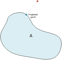
Projection onto a set means finding a point in the set that minimizes the distance to a given point.
Typically each constraint of your problem defines a set. If you have more than two constraints, there is a trick, called Divide and Concur, to combine them into two sets and perform regular DM.

I have implemented a Sudoku solver using this approach. Sudoku is a constraint satisfaction problem and fits to this approach with proper definition of constraints. Make sure to check it out here.


Let's define these approaches formally and build the basis for the Sudoku solver. I will skim over some of the details to keep things compact and casual.

Difference Map

Say you have two sets $A$ and $B$ and you can project a given point to these sets via functions $P_A(\cdot)$ and $P_B(\cdot)$.

A naive approach would be to select an initial point and project it onto $A$ and then $B$ and repeat the process until convergence. This procedure of applying a function repeatedly is often called fixed point iteration.
$$
x_{k+1} \leftarrow P_B(P_A(x_k))
$$This works if the sets are convex. If the sets are not convex, this fixed point iteration has no guarantees and fails to provide a solution most of the time. We can do better than that, consider:
$$
x_{k+1} \leftarrow x_k + P_A(2P_B(x_k)-x_k)-P_B(x_k)
$$ If this scheme ever converges (i.e. $x_{k+1} = x_k$), it means that $P_A(2P_B(x_k)-x_k)-P_B(x_k) = 0$. Following this $P_A(x_k) = P_B(x_k)$. This means that we have found point contained in both sets!

This is all very good, now let's introduce a hyperparameter to allow us to fine tune the algorithm for different problems.
$$
x_{k+1} \leftarrow x_k + \beta \left( P_A(f_B(x_k)) - P_B(f_A(x_k)) \right)
$$ where
$$
f_A(x) = P_A(x) - \frac1{\beta}(P_A(x) - x) \\
f_B(x) = P_B(x) + \frac1{\beta}(P_B(x) - x)
$$

We have just defined Difference Map algorithm. Note that the expressions above are equal to the previous expression for $\beta=1$.

Divide and Concur

To use DM you need to define your constraints as two different sets and you need to define projection operations onto those sets. Expressing your problem exactly as two sets might not be easy for every task. We need a way of using the same framework with many constraints.

Say, you have $N$ constraints and associated projection operations defined by these constraints $P_1(\cdot), P_2(\cdot), \dots, P_N(\cdot)$. Roughly, DC works in an $N$ times larger space. Say a point in this space is $x=(x_1 x_2 \dots x_N)$. $P_A(x)$ projects a given point onto $N$ different sets ($x_i$ to set $i$) and concatenates the results. $P_B(\cdot)$ averages them out at each step. More formally, we put together these different constraints together in a Difference Map framework by defining:
$$
\begin{align*}
P_A(x) &= \text{concat}(P_1(x_1), P_2(x_2), \dots, P_N(x_N)) \\
P_B(x) &= \text{concat}(\bar{x}, \bar{x}, \dots, \bar{x})
\end{align*}
$$ where $\bar{x}$ is the mean of $\{x_1, \dots, x_N\}$.

Solving Sudoku with Divide and Concur

We will represent Sudoku grid with a $9\times9\times9$ array, if the element at $(i,j,k)$ is $1$ that means there is a symbol $k$ in cell $(i,j)$. The rest is filled with zeroes.

Using this representation we have 4 constraints. We are familiar with three of the constraints, they are the very foundations of Sudoku: Each row, column and $3\times3$ block contains only one of each symbol. The fourth one is a little bit different, it is the direct result of the $9\times9\times9$ representation we use: there should be only single symbol at each cell. If we don't put this constraint we may have fractional symbols at each cell. For example we may have a solution where at a cell there is 0.7 "4", 0.1 "6" and 0.2 "9" (note that they sum up to 1).

Given a possibly fractional state $x$ the projection onto a $i^\text{th}$ row constraint is finding the configuration $p(j)$ that minimizes $-\sum_{j=1}^9 x_{ijp(j)}$. I won't give details to keep things simple, you can check out the original paper. This assignment problem can be solved quickly using the famous Munkres (a.k.a. Hungarian) algorithm.

Column and block constraints are very similar in their nature, the same approach can be used for them. For a cell, projection onto the set defined by symbol constraint is finding the symbol with minimum value in $-x$, in other words $\arg \min_k -x_{ijk}$ for cell $(i,j)$.

Solver in Action

Check out my DC implementation of Sudoku here. Source code is also available on github.

A MATLAB implementation is also available in the repository. I didn't realize how MATLAB makes life easier when you work with matrices until I started to port it into Javascript. I used math.js library but all the indexing and range operators didn't make life easier.

References

Elser, Veit, I. Rankenburg, and P. Thibault. "Searching with iterated maps." Proceedings of the National Academy of Sciences 104, no. 2 (2007): 418-423.
Gravel, Simon, and Veit Elser. "Divide and concur: A general approach to constraint satisfaction." Physical Review E 78, no. 3 (2008): 036706.

(Yapay) sinir ağı saçmalatmaca

, Friday 5 June 2015
Son dönemde derinlemesine öğrenme (deep learning) kavramı oldukça popüler. Bir çok problemde en güncel yapay öğrenme yöntemlerine hatrı sayılır derecede fark atıyor. Aslında fikir eski bir fikir, temelde yapay sinir ağlarından (artificial neural networks) hiçbir farkı yok. Bir ara gözden düşmüştü, hesaplama gücümüz ve konu hakkında anlayışımız ilerleyince camianın gündemine tekrar oturdu. Bu yapıları bu kadar güçlü yapan şey, sadece bir fonksiyonun parametrelerini değil, fonksiyonun kendisinin de en iyi olabilecek halini öğreniyor olması.

Bu yapılar alternatiflerine kıyasla baya becerikli, ses ve resim tanımada oldukça başarılılar. Örneğin milyonlarca resimde çok az hatayla aşağıdaki resimdekine benzer etiketlemeler yapabiliyor.

Deep learning tarafından etiketlenmiş bir resim. Kaynak: http://goo.gl/30neSn

Yapay sinir ağlarını ilk duyduğumda çok heyecanlanmıştım, hatta hala yapay bir bilinç üretilecekse buna benzer mekanizmalar yardımıyla gerçekleşeceğini düşünüyorum; aşırı basit bir sürü bileşenin etkileşimlerinin karmaşık davranışlar doğurması biçiminde. Bence illa ki yapay bilincin öğelerinin beyininkilere benzemesi gerekmiyor, altta yatan mekanizmayı çözmemiz yeterli. Benzer mantıkta, ürettiğimiz uçakların hiçbiri kuş gibi kanat çırparak havada ilerlemiyor.

Yakın zamanda yapılan bir kaç araştırma bu yapıların çok ciddi bir açığını keşfetti. Bu sinir ağlarının kör noktası var! Öyle ki, mesela yukarıdaki köpek resmini gözle ayırt edilemeyecek kadar değiştirip resimde aslında cep telefonu olduğuna ikna edebiliriz. Aşağıdaki resimde, soldaki resim ortadaki değişikliğe uğratılıp sağdaki resim elde ediliyor. Ve derinlemesine öğrenme sistemleri sağdakileri çok yüksek bir kesinlikle deve kuşu zannediyor!

Kaynak: http://arxiv.org/abs/1312.6199

Yakın zamanda yapılan başka bir çalışmada, bu derinlemesine öğrenme sistemlerine saçma sapan resimleri aslında bir şeylermiş gibi yutturabileceklerini gösteriyorlar. Aşağıda bu yapıların, özel yollardan üretilmiş abuk subuk resimleri nelere benzettiğinin bir örneği var:
Kaynak: http://arxiv.org/abs/1412.1897v4

Aslında bu zihin tutulmaları yapay sistemlere özgü değil. Hatta sanatın temelinde bu var. Çok iddialı girişimi biraz açayım. İstanbul'da yaşayanlarınız belki farketmiştir, bazı martıların gagalarının ucunda kırmızı bir leke vardır. Bilimadamları da oyuncak bir martı yapmışlar ona gaga takmışlar, bir de almışlar yavru bir martıyı koymuşlar sahte martının önüne. Gaga tertemizken yavru martı tepkisiz kalmış. Bilimadamları sahte gaganın ucuna kırmızı lekeden koyunca yavrucak annesinden yemek isterken yaptığı hareketlerden yapmaya başlamış.

Esas kopuş sahte gaganın üzerine noktasal kırmızı leke yerine 3 tane çizgi çekince yaşanmış. Yavru martı çıldırmış, sahte martının önüne gelip bir martı yavrusunun normalde sergilemeyeceği türde hareketler yapmış, dört dönmüş.
Dişi martı, sahte gaga, çıldırtıcı çekicilikte sahte gaga Kaynak: https://goo.gl/xCIuv9
Başka bir deyişle, doğal koşullarında oluşmayacak uyaranı sisteme yapay yollardan verince sistem saçmalayabiliyor. Tabi ki her yapay uyaran için bu geçerli değil, saçmalamaya yol açacak uyaranın bir şekilde sıradan uyaranla bağı var, ona benziyor. Ama, bu uyaranın tam olarak ne olabileceğini de çeşitlemeleri denemeden bilemiyoruz. Örneğin 3 kırmızı çizginin mi yoksa noktasal mavi bir lekenin mi daha büyük saçmalamaya yol açacağını test etmeden öngöremiyoruz.

Aslında sanat tam da bu mekanizmadan doğuyor. Zihnimiz kabaca belli girdilere belli çıktılar üretmeye yönelik çalışmak üzere bağlantılar içeriyor, tabi ki bu girdiler ve çıktılar biyolojik ve kültürel yollar ile şekilleniyor. Sanatçı bu bağlantıların şimdiye kadar hiç beklemediği olasılıkları keşfediyor ve bizler üzerinde çok acayip duygu durumları uyandırıyor.

Demem o ki, yapay sinir ağlarının kör noktaları aslında çok uzun zamandır bir arada yaşadığımız bir olgu. Hatta yapay bilincin bir şekilde sanat anlayışına sahip olmasını istiyorsak bu kör noktalar gerekli bile.

Probability of k collisions

, Friday 30 January 2015
While I was reading about hash tables I stumbled upon this deceptively simple question. I have rephrased it to make it easier to understand.
Say we have $m$ buckets. We select a random bucket and put a ball in it, we repeat this (select-put) $n$ times. In the end what is the probability of having at least one bucket with $k$ balls?
My initial attempts to solve it failed, and I posted the question on math.stackexchange. An approximation for large values of $m$ and $n$ was posted as an answer but I was interested in exact results. Once I realized I had no way of finding someone else's solution, I was able to solve it myself.

Simulation

First, to check if my solution is correct, I have written a small program to simulate the select-put procedure million times and report the experimental probability for different values of $m$,$n$ and $k$. If you are interested, you can find the java code at the end of my post.

Solution

First we will start with writing the probability of 1 box having $k$ balls. Then using inclusion-exclusion principle we will generalize. Let's write the probability of putting first $k$ balls into the first box and remaining balls to the other boxes: $$ \left(\frac1{m}\right)^k \left(1-\frac1{m}\right)^{n-k} $$ We have $\binom{n}{k}$ ways of putting $k$ balls into a particular box (e.g. first box), and we have $m$ such boxes. So the probability becomes: $$ m \binom{n}{k} \left(\frac1{m}\right)^k \left(1-\frac1{m}\right)^{n-k} $$ But the expression above suffers from double counting, i.e. it counts configurations that contains multiple boxes with $k$ balls more than once. So we need to subtract the value for 2 boxes having $k$ balls, add the value for 3 boxes having $k$ balls, etc... Let's write the probability of putting first $k$ balls into the 1st box, next $k$ balls into the 2nd box, and remaining balls to the other boxes. $$ \left(\frac1{m}\right)^k \left(\frac1{m}\right)^k \left(1-\frac1{m}\right)^{n-2k} $$ We have $\binom{n}{k}\binom{n-k}{k}$ ways of putting $2k$ balls into two particular boxes (e.g. first and second box), and we have $\binom{m}{2}$ such boxes. So the probability becomes: $$ \binom{m}{2}\binom{n}{k}\binom{n-k}{k}\left(\frac1{m}\right)^k \left(\frac1{m}\right)^k \left(1-\frac1{m}\right)^{n-2k} $$ At this point you should be able to see the pattern that is emerging.

Generalization

If we put together and generalize what we have done so far we get the following expression as probability of having a box with $k$ balls: $$ \sum^{\lfloor \frac{n}{k} \rfloor}_{i=1} (-1)^{i+1} \binom{m}{i} \left[ \prod^{i-1}_{j=0} \binom{n-jk}{k} \right] \left( \frac1{m} \right)^{ik} \left( \frac{m-i}{m} \right)^{n-ik} $$ The powers of $-1$ at the beginning enables adding values for odd number of balls and subtracting values for even number of balls, i.e. inclusion-exclusion principle.

The code

  private static double calculateKcollisions(int m, int n, int k) {
    double probability = 0;

    int sign = 1;

    for (int i = 1; n - i * k >= 0 && i <= m; i++) {
      double p = binomial(m, i) * pow(1.0 / m, i * k);
      p *= pow((double) (m - i) / m, n - i * k);

      for (int j = 0; j < i; j++) {
        p *= binomial(n - j * k, k);
      }

      probability += sign * p;
      sign *= -1;
    }

    return probability;
  }

Simulation code

  private static final Random RNG = new Random();

  public static void main(String[] args) {
    int sampleCount = 1000000;

    for (int experimentNo = 0; experimentNo < 10; experimentNo++) {
      int m = RNG.nextInt(7) + 3;
      int n = RNG.nextInt(m) + RNG.nextInt(10) + 1;
      int k = RNG.nextInt(n + 1);
      
      System.out.println(format("m:%d  n:%d  k:%d", m, n, k));

      int successCount = 0;
      for (int sampleNo = 0; sampleNo < sampleCount; sampleNo++) {

        int[] boxes = new int[m];

        for (int i = 0; i < n; i++)
          boxes[RNG.nextInt(m)]++;

        for (int i = 0; i < m; i++) {
          if (boxes[i] == k) {
            successCount++;
            break;
          }
        }
      }

      double experimental = (double) successCount / sampleCount;

      double calculated = calculateKcollisions(m, n, k);

      System.out.println(format("xperimental: %f  calculated: %f", experimental, calculated));
      System.out.println(format("diff: %.2f\n", abs(experimental - calculated)));
      System.out.println();
    }
  }

Blogger'a taşınıyoruz

Bir kaç ay önce anlak'ın koştuğu wordpress kurulumumun hack edilmiş olduğunu keşfettim. Biraz uğraştıysam da sistemde yarattıkları açıklardan tam anlamıyla kurtulamadım. Zaten ne zamandır sunucu idaresini kendi üzerimden atmak istiyordum. anlak'ı bu vesileyle Blogger'a taşıma sürecini başlattım.

anlak için temel ihtiyaçlarım şunlardı:
  • anlak.com altında yayın yapmak.
  • Eski linklerin korunması. stackoverflow gibi mecralarda kaynak niyetine gösterilmişti. oradan trafik akışını kaybetmek istemedim.
  • $\LaTeX$ ile matematik yazabilmek.
  • Kod renklendirme.
  • Temayı korumak.
  • Tüm bunların ücretsiz ya da minimum maliyetli olması.
Blogger tüm bunları ücretsiz sağlayabiliyordu. Şu an tek korkum Google Reader gibi fantastik bir ürünü kapattığı gibi bunu da kapatması.

Blogger'ın kötü yanı da var tabi. Temalar genellikle çok çirkin. Güya bazı şeyleri kolaylaştırmak için çok karmaşık bir tema dili yaratmışlar, bu yüzden güzel tema bulması çok zor. Ben anlak'ın varolan tasarımını uyarlayana kadar çok uğraştım, hala da biraz kalabalık var.

Şimdilik en çok ziyaret edilen sayfaları taşımakla başladım, yavaş yavaş tüm içeriği eklemiş olacağım. Bunca yıldır beni barındıran süpersonik kullandığın kadar ödeli hosting hizmeti nearlyfreespeech'e de pek müteşekkirim. RSS feedlerinizi de güncellemeyi unutmayın. Hadi, hepinize sevgiler.

Matlab'ın yeni çizim motoru: HG2

, Tuesday 24 June 2014
Geçenlerde yakında yayınlanacak Matlab 2014b'yi denemem için Mathworks'ten mail geldi. Yüklemenin ardından uzun süredir beklediğim HG2 çizim motorunu nihayet 2014b ile birlikte resmi olarak yayınladıklarını görünce çok sevindim. HG2 demek daha güzel grafikler demek. Hemen örnek bir grafik ile güzelliği gösterelim:


Üstteki eski Matlab ile, alttaki yeni HG2 motoru kullanan Matlab ile çizilmiş bir grafik. Ne kadar da hoş değil mi. İlk gözümüze çarpan değişiklik anti-aliasing varsayılan olarak açık ve (255,0,0) gibi uç renkler yerine daha pastel renkler kullanmışlar. Bunun dışında çizim için kullanılan renklerin sırası mavi, yeşil, kırmızı diye değil mavi, kırmızı, sarı diye gidiyor.

Bunun dışında HG2 ile birlikte grafikler için set() ve get() kullanmak da tarihe karışıyor. Grafiğin handle'larının özelliklerini kullanarak her türlü niteliğini değiştirebiliyorsunuz. Örneğin:
h = gca;
h.Title.String = 'HG2 Çok yaşa!';
h.Title.Color = 'b';
h.YRuler.Axle.LineStyle = 'dotted';

Yukarıdaki kod ile mavi renkte bir başlık ekledik. Ayrıca Y eksenini de düz değil de kesikli çizgiye dönüştürdük. Böylesi kod, eski stringly typed alternatiflerine göre çok daha güzel.


Matlab 2014b'ye erişimi olmayanlar için süper haberim var, eski Matlab sürümlerinde komut satırından -hgVersion 2 opsiyonunu belirleyerek deneysel HG2 mototrunu etkin hale getirebilirsiniz.


Yazının başında örnek grafikleri çizdirmek için kullandığım kod:
x = -4:0.01:4;
y = normpdf(x);

figure('pos',[100,100,300*1.6,300]);
hold all;

plot(x, y);

y = sin(x)/10 + 0.1;
plot(x, y);

ylim([-0.1 0.5]);
box off; grid on;

kaynak: Undocumented Matlab HG2 update